Growing a Lorenz Butterfly in R

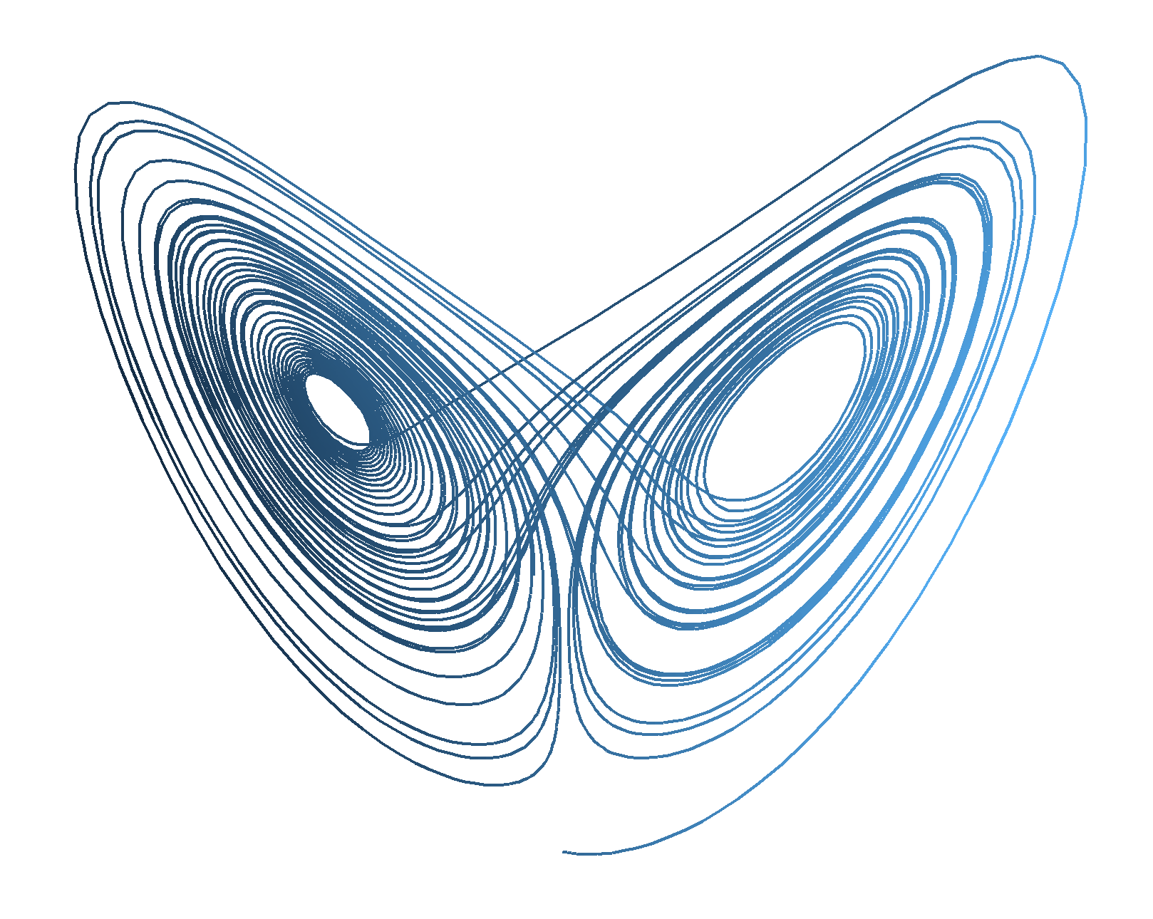
The Lorenz equations spawned the term ‘Butterfly Effect’. They are a set of mathematical equations that display chaotic behaviour (and produce some pretty graphs):

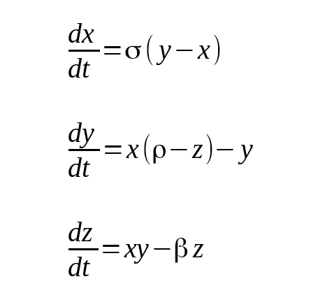
The equations model atmospheric convection for given starting states in x,y,z and for a set of constants σ, ρ, β. We’ll vary ρ and create an animated gif using R see how a Lorenz butterfly grows.

We’ll use deSolve to solve the equations and ggplot to create the plots.

library(deSolve)
library(ggplot2)

Let’s set up the parameters and initial states. The classic parameters are σ = 10, β = 8/3 and ρ = 28. We’re seeing how the butterfly grows as ρ varies so r (ρ) is a sequence.

parameters <- c(s = 10, b = 8/3)
r <- seq(0, 30, by = 0.05)
state <- c(X = 0, Y = 1, Z = 1)
times <- seq(0, 50, by = 0.01)

We define the Lorenz equations as a function for deSolve. This vignette describes the structure of the function.

Lorenz <- function(t, state, parameters) {
  with(as.list(c(state, parameters)), {
    dX <- s * (Y - X)
    dY <- X * (r - Z) - Y
    dZ <- X * Y - b * Z
    list(c(dX, dY, dZ))
  })
}

We can now run the solver for each value of ρ and keep the results in a list. I’ve chosen the Euler method because I know how to hand crank it.

out <- lapply(r,
              function(x){
                ode(y = state,
                    times = times,
                    func = Lorenz,
                    parms = c(r = x, parameters),
                    method = "euler")
                }
              )

Next we make our plots and save them to disk to turn into our animated gif.

imageStorePath <- '\\images\\lorenz_r\\'

plots_XZ <- list()
for(i in 1:length(r)) {
  p <- ggplot(data.frame(out[[i]])) + 
    geom_path(aes(x = X, y = Z, colour = Y)) +
    ggtitle(paste0('Lorenz attractor r = ', r[i])) +
    theme(
      axis.text.x = element_blank(),
      axis.title.x = element_blank(),
      axis.text.y = element_blank(),
      axis.title.y = element_blank(),
      axis.ticks = element_blank(),
      panel.background = element_blank(),
      legend.position = "none")
  
  ggsave(filename = paste0(imageStorePath, sprintf('%05.2f', r[i]), '.png'),
         plot = p, 
         device = 'png') 

  plots_XZ[[i]] <- p
}

A system call to ImageMagick’s convert makes our animated gif. This isn’t the most efficient way, but it works…

imageMagick <- '"C:\\Program Files\\ImageMagick-7.0.7-Q16\\convert.exe"'

system(paste0(imageMagick, ' -loop 0 -delay 10',   # call imageMagick

              paste0(' ', imageStorePath, '*.png '),
              ' -layers Optimize ', # compress the gif

              imageStorePath, 'lorenz_XZ_vary_r.gif'))

Finally we tidy up our intermediate images.

for (i in 1:length(r)){
  file.remove(paste0(imageStorePath, sprintf('%05.2f', r[i]), '.png'))
}

Thanks for reading.