Classifying Cookies

In this post we’ll use data from a supemarket website to classify products, as either cookies or crisps.

I’m boring enough to spend my free time classifying supermarket data, but not boring enough to manually build a data set, so I wrote this code to grab the data. You can run it yourself or you can download the result here.

The data has unit price, price per quanitity, ingredients and nutrition information. We will figure out a few more features, but I don’t want this to be a feature building exercise. I generally expect cookies to be heavier, more expensive and have more ingredients.

We load in our libraries and the data.

library(class)
library(gmodels) # for CrossTable

library(caret)
library(MLmetrics) # for custom summary functions


library(reshape2)
library(dplyr)

library(ggplot2)

inDat <- readRDS('C:\\Users\\Chris\\Documents\\Data\\cookie_classifier\\cookies_and_crisps.Rds')

Reshape the data so it’s easier to use.

numIngredients <- unlist(lapply(inDat, function(x) length(x['ingredients']$ingredients)))
prices <- unlist(lapply(inDat, function(x) as.numeric(gsub("\\£", "", x$unitPrice))))
type <- unlist(lapply(inDat, function(x) x['searchTerm']))

perUnit <- unlist(lapply(inDat, function(x) x['perUnit']))
perQuantity <- unlist(lapply(inDat, function(x) x['perQuantity']))
pricePer <- unlist(lapply(inDat, function(x) as.numeric(gsub("\\£", "", x$pricePer))))

Figure out how much something costs per gram.

priceGram <- cbind.data.frame(pricePer, perQuantity)

ingredientPrices <- cbind.data.frame(numIngredients, prices, type, perUnit, pricePer)

ingredientPrices$pricePerGram <- unlist(
  apply(ingredientPrices, function(x){ ## this adds a list to the df

    if(x['perUnit'] == 'g'){
      as.numeric(x['pricePer']) / 100
      }else if(x['perUnit'] == 'kg'){
        as.numeric(x['pricePer']) / 1000
        }else {
          NA
        }
    }, MARGIN = 1
    )
  )

ingredientPrices <- ingredientPrices[, c('numIngredients', 'prices', 'type', 'pricePerGram')]

set.seed(1758952857)

Then we figure out the weight.

ingredientPrices$weight <- ingredientPrices[, 'prices'] / ingredientPrices[, 'pricePerGram']

We’ll build a kNN. To do this we randomly split our data into training and testing samples.

# remove NA pice per grams for KNN later on

naPricePerGram <- !is.na(ingredientPrices$pricePerGram) 
ingredientPricesValid <- ingredientPrices[naPricePerGram, ]

trainInd <- sample(seq_len(nrow(ingredientPricesValid)), size = (0.7 * nrow(ingredientPricesValid)))
trainSet <- ingredientPricesValid[trainInd, ]
testSet <- ingredientPricesValid[-trainInd, ]

setSelection <- cbind(ingredientPricesValid[trainInd, ], set = 'train')
setSelection <- rbind(setSelection, cbind(ingredientPricesValid[-trainInd, ], set = 'test'))
setSelection <- rbind(setSelection, cbind(ingredientPricesValid, set = 'all'))

setProp <-as.data.frame( prop.table(table(setSelection[, c('type', 'set')]), margin = 2))

We can check that the split is representative of the full data of 95 cookies and 216 crisps.

ggplot(setProp) + 
  geom_bar(aes(x = set, y = Freq, fill = type), position = 'stack', stat = 'identity') +
  labs(y = 'Frequency') +
   theme( 
     axis.title.x = element_blank(),
     legend.title = element_blank(),
     panel.background = element_blank())

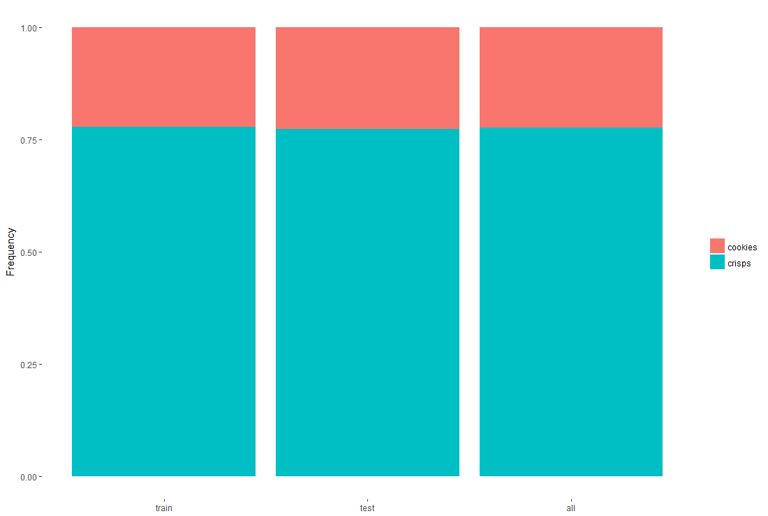
The test set has a few more cookies than the full set, but it looks good enough for us.

We then train the model on, the number of ingredients, price and weight. I’ve set the model to look at the 5 nearest neighbours. Considering our data only contains ‘cookies’ and ‘crisps’ a tie should be impossible.

kNN <- knn(trainSet[, c('numIngredients', 'prices', 'weight')], 
testSet[, c('numIngredients', 'prices', 'weight')],
           trainSet$type, l = 0, k = 5, prob = T)

accuracy <- cbind(testSet, kNN)

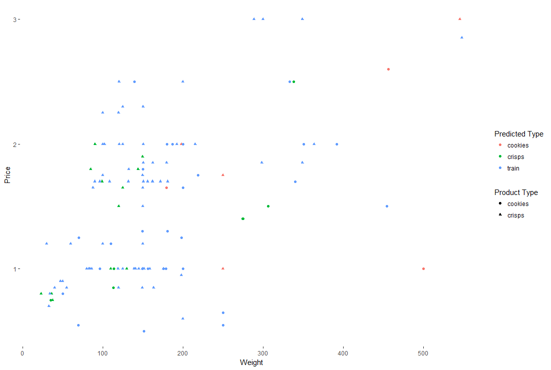
kNNPlotDat <- rbind(accuracy, cbind(trainSet, kNN = 'train'))

We can get a feel of our result below. Red circles and green triangles are correct classifications. I’ve added the training data in blue so we can see the full data set.

ggplot(kNNPlotDat) + 
  geom_point(aes(x = weight, y = prices, shape = type, colour = as.factor(kNN))) +
  labs(x = 'Weight', y = 'Price', colour = 'Predicted Type', shape = 'Product Type') +
  theme(panel.background = element_blank(),
        legend.key = element_blank())

I was hoping we would see cookies (a bigger, heavier so presumably more costly product) form a cluster of high price but unfortunately, we do not.

We can compare the result of the classifier with the true classification to see how accurate we are.

nrow(accuracy[accuracy$type == accuracy$kNN, ]) / nrow(accuracy)

0.786

Is this accuracy good? Not really, if we just assumed everything was crisps we’d do about as well as the model.

prop.table(table(accuracy$type))

cookies = 0.226

crisps = 0.774

You might think comparing to more neighbours will improve the accuracy, so I wrote a bit of code that varies the number of neighbours to check.

We’ll compare models that use between 1 and 30 neighbours.

k <- 1:30

I want to check the overall accuracy of the model, as well as how many cookies or crisps it gets right, regardless of false matches.

CookieCrispRecall <- function(data, lev = NULL, model = NULL){
  
  # please excuse the hardcoding

  cookieRecall <- nrow(data[(data$obs == data$pred) & 
  (data$obs == 'cookies'), ]) / nrow(data[(data$obs == 'cookies'), ])
  
  crispRecall <- nrow(data[(data$obs == data$pred) & 
  (data$obs == 'crisps'), ]) / nrow(data[(data$obs == 'crisps'), ])
  
  accuracy <- nrow(data[data$obs == data$pred, ]) / nrow(data)
  
  c(cookie = cookieRecall, crisp = crispRecall, model = accuracy)
}

We use the caret package to split the data into a set of 10 groups, each group then takes a turn as the test set. We repeat this 5 times and take the average for each number of nieghbours we’re testing.

ctrl <- trainControl(method = 'repeatedcv', number = 10, repeats = 5, 
summaryFunction = CookieCrispRecall, savePredictions = 'final')#, returnData = T)


knnFit <- train(type ~ ., data = ingredientPrices[, (names(ingredientPrices) != 'perUnit')], 
method = 'knn', trControl = ctrl, tuneGrid = as.data.frame(k), metric = 'model', na.action = na.omit, 
preProcess = c('center', 'scale'))

We then do a small reshape and plot to see how accurate the model is for how many nearest neighbours are used.

moltenIteratedKnn <- melt(as.data.frame(knnFit$results[, 1:4]), id.vars = 'k', 
variable.name = 'type', value.name = 'accuracy')

ggplot(moltenIteratedKnn) + geom_line(aes(x = k, y = accuracy, colour = type)) +
    labs(x = 'Neighbours', y = 'Accuracy', colour = '') +
  theme(panel.background = element_blank(),
        legend.key = element_blank())

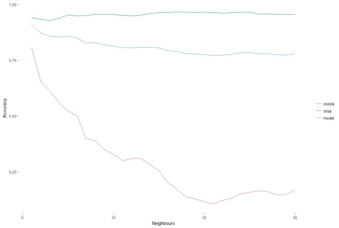
The lines for cookies and crisps show the proportion of each that were classified. If we predicted all cookies and crisps correctly, everything would have an accuracy of 1. If we just said everything is a cookie, our accuracy for cookies would be 1, crisps would be 0 and the accuracy of the model would be somewhere between.

We see the model is best at k = 1. When we use more neighbours the model generally gets better at finding crisps at the expense of finding cookes and reduces the models overall accuracy ie. it’s incorrectly flagging cookies as crisps.

I’m very suspicious at how good k = 1 looks. It could be because there are many more crisps than cookies and the data isn’t particularly ‘clustered’ (I hoped that cookies would give a cluster in high price, heavy weight to examine). This would mean adding more neighbours to the model simply finds more crisps and so an item is less likely to be predicted as a cookie.

With hindisight I went straight to a solution for the sake of a snappy post title. I should have spent more time exploring and understanding the data before trying to classify cookies, but for now, thanks for reading.