Bifurcation in Lorenz Equations
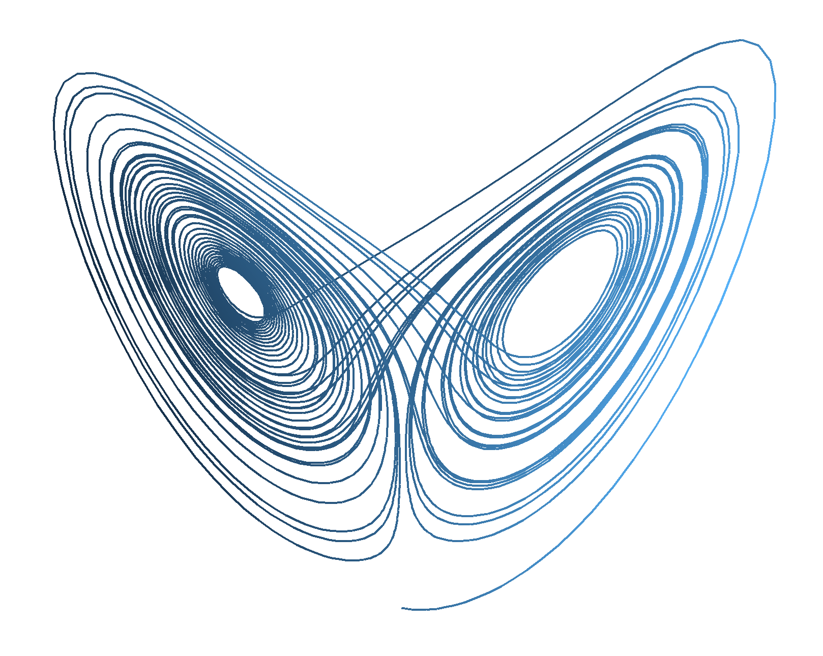
In Growing a Lorenz Butterfly in R we used the Lorenz equations to plot this butterfly.
The equations describe how a point moves around in 3 dimensions, they contain parameters which define the geometry of the 3 dimensions. With certain values the parameters create a geometry with deep valleys that the point quickly falls into, and with other values they create complex points of attraction that make the point endlessly loop around, never repeating the same path.
We changed one of the parameters and created an animation to see how the output changed. This post will examine a few settings of the parameter a bit more.
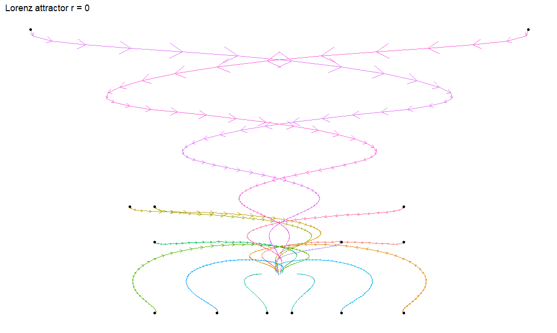
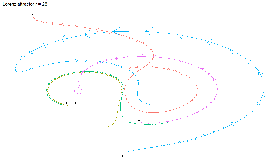
When we have a low value for one of the paramters, the plot has one center of attraction. I’ve dropped a few points around the attractor so we can see how it behaves. Imagine each black dot is a spring of water and the different cloured lines are rivers flowing around valleys. Everything works its way towards the attractor, no matter where it starts.
Setting the parameter to something bigger, we see a complex shape where 2 nodes of attraction fight each other and our starting points loop and swirl around the attractors. Our valley metaphor gets a bit weird, so please don’t take it too literally.
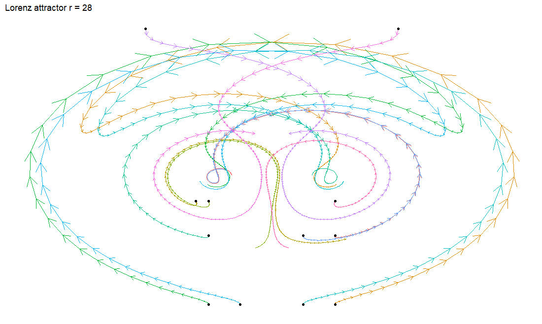
The plot is symmetric so I’ve removed some of the points to make it a bit easier to follow.
At the top we see a point that swoops towards the right hand attractor to orbit it before heading over to the left attractor. Below this we have two points that start near each other but soon follow drastically different paths. This is a classic example of chaos. I’ll let Jeff Goldblum explain it to you.
I’ve given a very qualitative description on the outputs of the equations. This is necessary because of the mathematically ‘unsolvable’ nature of the equations. If we think about an equation of motion (speed now = initial speed + acceleration x time) we can give it a set of starting conditions (initial speed, acceleration) and instantly know everything there is to know for all time. If we know the initial speed is 10 mph and the speed increases by 1 mph each second, then after 1 second the speed is 11 mph, after 2 seconds it’s 12 mph and after 100 seconds is 110 mph.
With the Lorenz equations
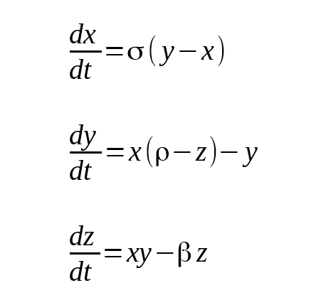
we know that our ‘speed’ (or temperature, convection, … etc) start with values (x, y and z) and change at some rate (dx/dt is the how we describe a rate of change in maths). The rates of change depend on the parameters which describe our geometry (σ, ρ and β) and where the values (x, y and z) currently are. This creates a complicated inter-dependence between the values governing the change in the rate of change. To figure out a value for a new time we have to ‘step through’ the calculations for intermidate time steps. To find the value of x after 100 seconds we must first calculate x after one second, we take this result and use it to calculate x after 2 seconds and so on.
How do we explore this a bit more methodically?
To help us see how changing the parameter ρ changes the geomtery of the valleys I dropped in one starting point and stepped through the equations. I then took the end of the result and squashed the values onto an axis.
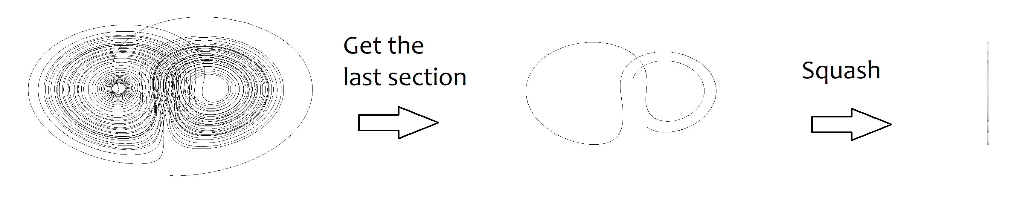
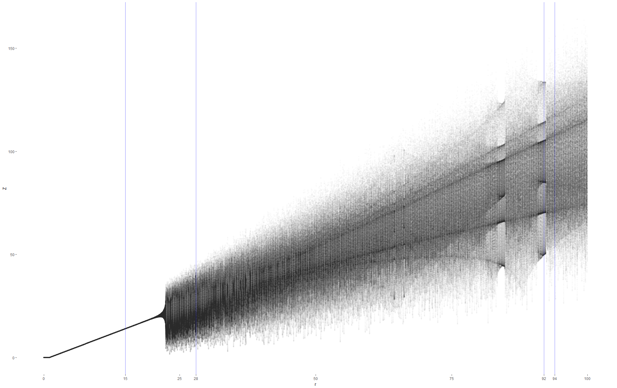
I repeated this for a range of values for the parameter ρ, and stacked them next to each other on the ‘bifurcation’ plot below.
Towards the left we see that the model is stable for the parameter. When the model settles down all the points are very close to each other, when we squash them we get a single point, as the paremeter changes this is represented as a neat line.
On the right, when the paremeter gets bigger, solutions become chaotic. They never settle down and squashing the plot gives us a blurred band. The band develops and we get dark lines running through it.
I’ve used blue lines to highlight some values for the parameter and shown thier full plots below.
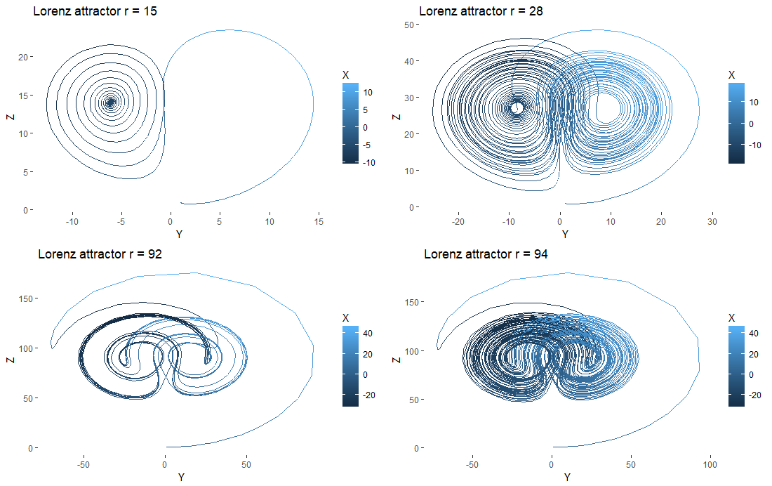
When ρ is 15, our starting point loops around one node of attraction in positive y before converging to a stable node at negative y. If we tested the bifurcation of y on ρ we’d see a branch in the plot. For ρ at 28 we see a broad butterfly which becomes a blurred band in the bifurcation plot, which is a classic sign of chaos. At ρ 92 the plot tightens up and we get white space in the bifurcation diagram before it loosens up again at ρ 94.
Thank you for reading.